Small Language Model

With the rise of generative AI systems like OpenAI's ChatGPT or Google's Gemini, I've become particularly interested in how they actually work. A quick search reveals that these systems are built on what's called a 'large language model' or LLM for short. An LLM is essentially a huge neural network, which is a mathematical model inspired by biological brains, that can be trained on massive amounts of data to acquire a sort of 'natural understanding' of what it's shown. Neural networks are used for things like classification of handwritten letters, face detection in images, and of course, language prediction in the case of LLMs.

But even knowing that, the question remains, how exactly do you go from an input string like 'I will' to some more or less sensical continuation like 'fight for you'? To explore this, I build what I call a 'small language model' or SLM for short. Basically all the peripheral steps are the same or similar to what you would do with an LLM, just the actual core is based on Markov chains instead of neural networks. Immediately one can infer some major limitations from that, but more on that later. For now, please enjoy this little demonstration I put together.

uniqueness:  ---

High-Level Overview

At a high level, the whole system can be split into two major parts. First, the training of the model: This is where it 'learns' from existing data (in our case pre-written text). Second, the generation using the trained model: This is where the model takes an input (a seed string) and produces a continuation based on what it learned. However, at no point does the model actually handle bare text. Instead, everything is broken down into smaller parts, called token. A token can be anything from multiple words to a single character. Try clicking the 'toggle token' button in the demonstration above to see exactly how text is split.

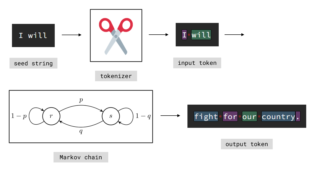
Conceptual generation process of a SLM.

To generate a fitting continuation of 'I will' the model performs two simple steps. First it splits the input into a list of token (in our case mostly words), to get ['i', 'will']. Next it finds whether any of these token (starting from the right) form a valid state of its Markov chain. If so, the model can simply 'walk the chain' to generate as many output token as needed, one at a time. That's how it might output something like ['fight', 'for', 'our',...] and so on.

Understanding the training process requires looking at how a Markov chain can even 'learn' to predict token sequences. Recall, a Markov chain is a stochastic process \(X_\mathbb{N} \subset S\), with its state space \(S\), such that \[ P(X_{n+1} = s \,|\, X_n,\ldots,X_1) = P(X_{n+1} = s \,|\, X_n) \] holds for all \(s \in S\). This means the chain only cares about its current state and not how it got there, which is both its biggest strength and its biggest limitation. If the state space is enumerable i.e. \(S = \{s_1,\ldots,s_m\}\) we define the transition probabilities \[ p_{ij} := P(X_{n+1} = s_j \,|\, X_n = s_i)\,. \] Notice how technically \(p_{ij}\) depends on \(n\), however in many applications (including ours) this is undesired. We therefore assume \(p_{ij} = \textit{const. } \forall n\) and call this property (time-)homogeneity. Finally all these probabilities are collected in a matrix \(\mathbb{P} := (p_{ij})_{ij}\) called the transition matrix. So how does this allow to 'learn' probable token succession? Consider this training text (from the model president-3, trained on U.S. inauguration speeches):

TXT
                        My fellow citizens: I stand here today humbled 
                        by the task before us, grateful for the trust 
                        you have bestowed, mindful of the sacrifices 
                        borne by our ancestors.
                    
First sentence of Obama's inauguration speech 2009.

To build a Markov chain we need two things: Its state space \(S\) and its transition matrix \(\mathbb{P}\). The state space naturally arises from tokenizing the training text (go ahead and try it) and treating each unique token as a state i.e. S = ['my', 'fellow', 'citizens', ...]. For the transition matrix we need to find the transition probabilities \(p_{ij}\) between states \(s_i, s_j \in S\). Since we assumed \(X_\mathbb{N}\) to be homogenous it holds \[ p_{ij} = \frac{\#(s_i \to s_j)}{N-1} = \frac{\omega_{ij}}{N-1} \] where the weight \(\omega_{ij} := \#(s_i \to s_j)\) is the number of times token \(s_i\) is followed by token \(s_j\) and \(N := \#S\) is the total number of unique token. Computing these weights is the training. A simple way to do so, is to first tokenize the input text and then iterate over the resulting token list as follows.

PSEUDO
                        token = split input text
                        for i = 1,...,N do:
                            // find correct transition 
                            indexA = index of token[i-1] in S
                            indexB = index of token[i] in S
                            
                            // update corresponding weight
                            weight[indexA][indexB] += 1
                    
General idea for training in pseudocode.

In our current example the first few weights are weight['my']['fellow'] = 1, weight['fellow']['citizens'] = 1. Because we're only dealing with the first sentence, each weight is only 1. However, if later parts of the text contain a certain passage again, we would bump up the corresponding weight to 2 and so on.

Tokenizer

Appearing both in training and generation, the tokenizer acts as the translation layer between human and model. Despite its importance the actual logic behind it is quite simple: Define a list of characters that seperate token e.g. separator = [' ', '\n', '\r'], and a list of special token that should be recognized on their own e.g. special = ['.', '!', '?']. Then parse the input text one character at a time. Whenever a separator or a special character is reached, the current sequence of characters becomes a token, and the process continues. By repeating this until the end of the text, it is converted into a clean sequence of token.

Tokenizer algorithm at work.

The actual code introduces a Tokenizer class with fields for separator and special. The described algorithm is then implemented in the method Tokenizer.split. I decided to simplify/skip some non-essential details, to keep the presented code focused and easy to follow. Omitted sections are marked with /**/ starred comments, while temporarily hidden parts are shown as ... triple dots.

JS
                        Tokenizer.split = function(input) {
                            /* clean up input first */
                            const output = []; let token = '';

                            // pushes current token then resets it
                            const flush = (str) => {
                                if (!str.length) return;
                                output.push(str); token = '';
                            };

                            // builds up token and checks when to flush
                            for (const char of input) {...}
                            return output;
                        }
                    
High level from string input to token output.

A small helper function flush, pushes the current string into the output array (recognizing it as a token) and then clears the temporary buffer. With that in place, the actual algorithm becomes super clean: Simply flush whenever either a separator or a special character is encountered. If the character is special, flush it as a token as well. Otherwise, just continue building up characters until the next flush point.

JS
                        for (const char of input) {
                            /* skip ignored characters */
                            const fullWord = separator.includes(char);
                            const specChar = special.includes(char);

                            // special chars form token on their own
                            if (fullWord || specChar) flush(token);
                            if (specChar) flush(char);
                            
                            if (!fullWord && !specChar) token += char;
                        }
                    
Implementation of tokenizer algorithm.

Hashmap

Next we'll cover the concept of a hashmap. A hashmap is a data structure that enables extremely fast lookups, even when handling millions of elements. This will later be crucial for keeping our Markov chain efficient. JavaScript already provides a built-in version of this via new Map(), however creating one ourselfs is much more fun. The basic idea is simple: Instead of storing all elements in a single large bucket, store them in many small ones with only a few elements per bucket. Combining this with a way of quickly determining which bucket an element belongs to, we only need to search a few elements instead of all of them.

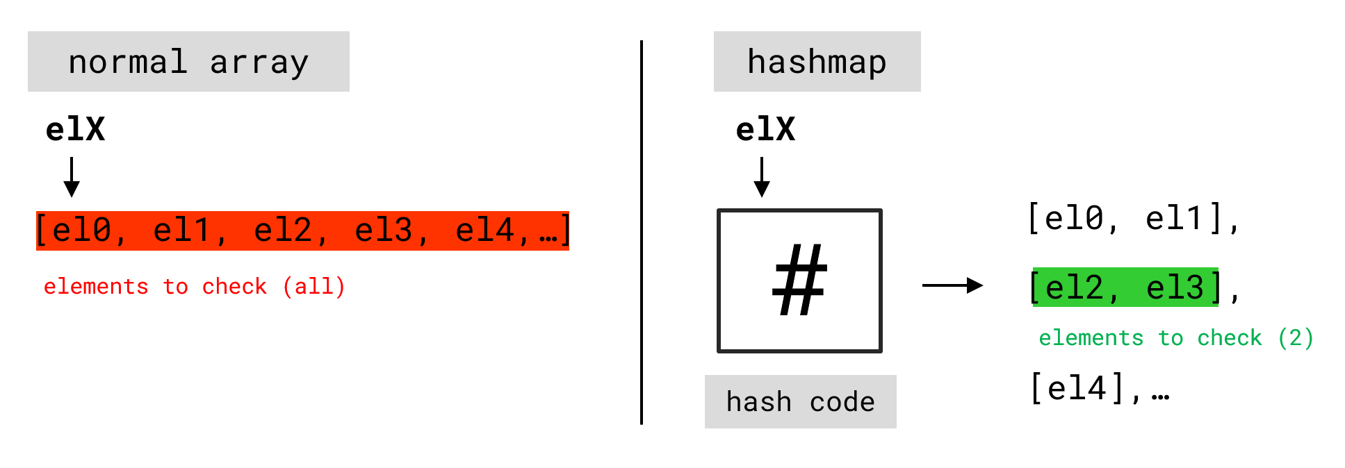
Classic array vs. hashmap.

The core component of a hashmap is the so-called hash function. For our purposes, a hash-function \(h: \mathcal{X} \to \mathbb{N}\) is a mapping between \(\mathcal{X}\), the set of all possible strings given some alphabet \(A\), and \(\mathbb{N}\) (in practice often restricted to 32-bits, for example). The value \(h(\chi)\) is called the hash code of string \(\chi\). There are many different ways to define such a function. For instance \[ h(c_1 \cdots c_n) := \sum_{k \leq n} \iota(c_k) \] where \(\chi = c_1 \cdots c_n\) is represented by its characters and \(\iota: A \to \mathbb{N}\) is an embedding of the given alphabet into \(\mathbb{N}\) (e.g. using ASCII codes). However, not all hash functions are equally effective. Different applications prioritize different properties. In the context of hashmaps, we typically want a low collision rate, meaning \(h\) should be as close to injective as possible, and a high spread characteristic, meaning \(h(\chi)\) should be distributed approximately uniformly over its range when \(\chi\) is uniformly sampled. These two properties ensure that a hashmap distributes elements evenly among its buckets.

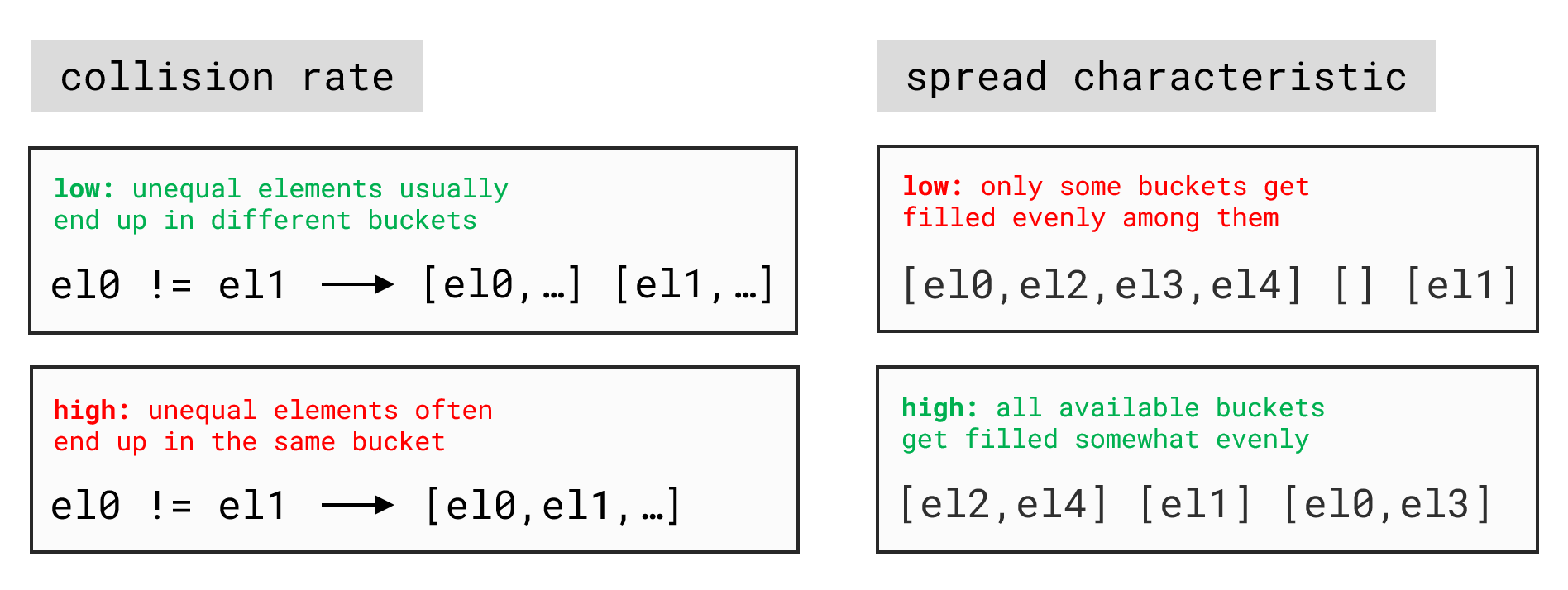
Collision and spread are related but not the same.

As our hash function, we'll implement the DJB2a hash, named after its inventor, the American mathematician Daniel J. Bernstein. Similar to the previous example, the hash relies on an embedding \(\iota\), in this case UTF-16 codes (JS specific). We define two constants \(h_0,\,\lambda\) and compute for each \(c_k\) input character \[ h_k := \lambda h_{k-1} \oplus \iota(c_k) \] where \(\oplus\) denotes the bitwise XOR operator (the original version used addition, but XOR was found to give slightly better distribution). The final hash is then given by \(h(c_1 \cdots c_n) := h_n \text{ mod } 2^{32}\). Bernstein determined the optimal constants \(h_0 := 5381\) and \(\lambda := 33\). While these were originally tuned for C-strings using 8-bit ASCII, they perform decently for our UTF-16 case as well. The so obtained hash function has both low collision rate and high spread.

JS
                        Hashmap._hashDJB2a = function(string) {
                            let hash = 5381;
                            for (let i = 0; i < string.length; i++) {
                                // multiply by 33 via left shift
                                hash = (hash << 5) + hash;
                                hash ^= string.charCodeAt(i);
                            }

                            // modulo 2^32 via unsigned right shift
                            return hash >>> 0;
                        }
                    
Efficient implementation of DJB2a hash.

While the implementation overall is fairly straightforward, two clever details are worth noting. First, multiplying by \(33\) can be done efficiently by shifting left by \(5\) bits (equivalent to multiplying by \(2^5 = 32\)) and then adding the original value once. Second, taking the remainder modulo \(2^{32}\) simply forces the hash to an unsigned 32-bit integer, which in JavaScript can be achieved with the unsigned right shift hash >>> 0.

From this we can introduce the Hashmap class, which uses the field _map to store all available buckets. As before, only key parts of the implementation are shown for clarity. Finding an element, given as key-value pair (ID, el) that matches a specific test function can be done in \(\mathcal{O}(1)\) time by first hashing the given ID and then simply searching the corresponding bucket.

JS
                        Hashmap._index = function(ID) {
                            let index = this._hash(ID);

                            // modulo 2^k via bitwise and
                            index &= (1 << this._power) - 1;
                            return index;
                        }

                        Hashmap.find = function(ID, match) {
                            /* make sure ID is valid first */
                            return this._map[this._index(ID)].find(match);
                        }
                    
Indexing and finding elements.

By keeping the size of _map as a power of \(2\), we can efficiently calculate the remainder modulo _map.length. To do so we take the bitwise AND between the current index and the map size (given as 1 << this._power) minus \(1\). This can easily be shown.

Proof. Let \((x)_2 = x_{n} \cdots x_1\) be an \(n\)-bit integer written in base \(2\). Then taking the remainder modulo \(2^k\) for \(k \leq n\) simply gives the lower \(k-1\) bits \(x_{k-1} \cdots x_1\). Equivalently \[ x \wedge (2^k - 1) \,=\, x_{n} \cdots x_1 \wedge 0 \cdots 0 \underbrace{1 \cdots 1}_{k-1\,\text{times}} =\, x_{k-1} \cdots x_1 \] where \(\wedge\) denotes the bitwise AND operator, since \(x_i \wedge 0 = 0\) while \(x_i \wedge 1 = x_i\). \(\square\)

Next we'll look at how elements are added to the hashmap. At first glance this seems straightforward. Just hash each ID and insert the element into its corresponding bucket. However, to ensure lookups can be done in \(\mathcal{O}(1)\) time it is crucial that all the buckets stay small. Therefore we define the load factor \[ \alpha := N \cdot 2^{-k}\] where \(N\) is the total number of stored elements and \(k\) is the current power of the hashmap (i.e. \(2^k\) is the total number of buckets). Since our hash function has both a low collision rate and a high spread, \(\alpha\) approximates the average fullness of the buckets. When adding a new element, we must check whether the load factor exceeds a defined maximum (typically \(0.7\)). If it does, we have to trigger a resize, which doubles the number of buckets (i.e. increment \(k\)) and rehashes all existing entries.

JS
                        Hashmap.add = function(ID, el) {
                            this._map[this._index(ID)].push(el);
                            this._total += 1;

                            // trigger resize if N / M > alpha_max where
                            // N = total elements and M = total buckets
                            const load = this._total / (1 << this._power);
                            if (load > this.alpha) this._resize();
                        }
                    
Adding an element might trigger a resize.

Markov Chain

As discussed, a Markov chain is defined by its state space \(S\) and the transition probabilities \(p_{ij}\) between those states. One way to think about this is a directed graph \((V,E)\), where each vertex represents a state \((V = S)\) and each edge \(e_{ij} \in E\) connects the \(i\)-th state to the \(j\)-th one with the weight \(\omega_{ij} = (N-1)p_{ij}\). This perspective not only works perfectly as the foundation for our implementation, but also provides a clear and intuitive way to visualize the structure of the chain.

Walking the chain (only non-zero weights are shown).

To implement this structure, we begin by introducing two classes: Edge and Vertex. An edge simply stores its weight and what vertex it's pointing to via targetID. Similary, a vertex holds its own ID along with a list of all outgoing _edges. However, the latter requires a bit more care. When adding edges we must ensure each one is unique. Otherwise the existing edge's weight should just be updated accordingly.

JS
                        Vertex.addEdge = function({ targetID, weight = 1 }) {
                            /* update total weight */
                            // if edge already exists just update weight
                            let edge = this._findEdge(targetID);
                            if (edge) { edge.addWeight(weight); return; }
                            
                            // else create new edge and add it to _edges
                            edge = new Edge({ targetID, weight });
                            this._edges.push(edge); 
                        }
                    
Adding edges requires us to ensure uniqueness.

From here we can introduce the Chain class, which consists of four main components: Two fields _state and _vertices, as well as two methods addVertex and nextState. Of course, there is much more to it (some of which we'll cover in later sections, though not all) so I encourage you to explore the full implementation on GitHub. The two fields are fairly straightforward: _state holds the vertex object corresponding to the current state of the Markov chain, while _vertices is an instance of our custom hashmap class containing all vertex objects that make up the chain's state space. As for the methods, similar to Vertex.addEdge adding a vertex to the chain requires us to ensure uniqueness. Otherwise the existing vertex's edges should, again, just be updated accordingly.

JS
                        Chain.addVertex = function({ ID, edges = [] }) {
                            // if vertex already exists just update edges
                            let vertex = this._findVertex(ID);
                            const update = edge => vertex.addEdge(edge);
                            if (vertex) { edges.forEach(update); return; }

                            // else create new vertex and add it to _vertices
                            vertex = new Vertex({ ID });
                            const create = edge => vertex.addEdge(edge);
                            edges.forEach(create);

                            this._vertices.add(ID, vertex);
                        }
                    
Adding vertices also requires extra care.

Notice how both, updating and creating an edge, simply mean to call addEdge, since that method already handles both cases automatically (a similar dynamic will reappear later once we discuss training). Now for the method that makes the magic happen: nextState advances the chain's current state to a randomly chosen connected one, considering their weights. This process is often referred to as 'walking the chain'. To make it happen, first select a random pivot between \(0\) and \(\sum_j \omega_{ij} - 1\) the total weight of all outgoing edges minus one. Next iterate over each outgoing edge and sum up their weights in a threshold variable. Once the threshold exceeds the pivot set the current edge's target as the new state.

JS
                        Chain.nextState = function(/* --- */) {
                            /* handle undefined state */
                            /* define random integer */
                            const pivot = randInt(this._state.weight);
                            let threshold = 0;
                            
                            // pick random edge according to their weights
                            // and advance current state to target vertex
                            for (const { weight, targetID } of this._state.edges) {
                                // update threshold with weight then check pivot
                                if ((threshold += weight) > pivot) {
                                    this._state = this._findVertex(targetID);
                                    return this._state;
                                }
                            }
                        }
                    
Selecting a new state by summing up weights.

Training & Generating

Before moving on, we'll introduce a concept called context depth. So far, we've only discussed handling sequences of individual token. If you try setting the context depth in the demo to 'low' and generate some text, you'll notice that much of it turns out to be semantic nonsense. However this is expected, as a simple Markov chain has no ability to 'learn' anything beyond statistical token succession. Still, a simple generalization of what we've done so far can help mitigate this limitation.

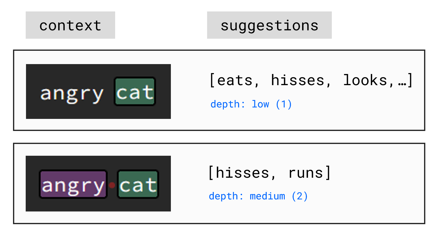
Deeper context allows for better suggestions.

Instead of treating each unique token as an individual state, we can group multiple token together to form a single state. For example, where a simple training text like 'the curious rabbit' would previously produce a Markov chain of [the]\(\,\to\,\)[curious]\(\,\to\,\)[rabbit], using a context depth of two yields [the,\(\,\)curious]\(\,\to\,\)[curious,\(\,\)rabbit] . Introducing this concept to our code luckily only requires that IDs can now be arrays of strings rather than single ones. For example, if you read carefully, you may have noticed that while discussing our Hashmap class, we introduced a _hashDJB2a function, but never actually called it. Instead, we used _hash, which is a simple wrapper capable of handling arrays of strings.

JS
                        Chain._depthID = function(token, depth, i) { 
                            return token.slice(i, i + depth); 
                        }
                    
Generalized IDs consist of multiple token.

Training a complete model therefore involves creating multiple Markov chains with different context depths. To build up a chain, first tokenize the input text and then iterate over the resulting token list. At each step, add a vertex of depth many token, with an edge pointing to the next vertex shifted one position to the right. Do this until the final vertex corresponds to the end of the token list.

JS
                        Chain.trainFrom = function(token, depth = this.depth) {
                            /* handle mismatched depth */
                            const train = (depth) => {
                                const ID = (i) => this._depthID(token, depth, i);
                                
                                // iterate token list and create vertices accordingly
                                for (let i = 0; i < token.length - depth; i++) {
                                    const edges = [{ targetID: ID(i + 1) }];
                                    const vertex = { ID: ID(i), edges };
                                    this.addVertex(vertex);
                                }
                            }

                            // create a separate markov chain for each depth
                            do train(depth); while (--depth > 0);
                        }
                    
Training chains with different context depths for one model.

Notice that, similar as before, we don't need to worry about whether a given vertex already exists. Updating and creating a vertex are both handled automatically by addVertex. To save a trained model, we store its vertices (the hashmap) as a compressed JSON file (.json.gz). To load it, simply decompress that file and read its content back into the _vertices field of a Chain instance. Click here to download all four of my trained models.

Generating output token from a given list of seed token is done by first deriving an initial state from the seed and then repeatably calling nextState().ID.last(). Since states can now contain multiple token, the actual next output is always the last element of the state's ID. While this procedure may appear straightforward, its implementation is somewhat more involved. Conceptually however, it can be divided into three parts, as shown below.

JS
                        Chain.generate = function(
                            { seed, length, depth = this.depth, /* --- */ }
                        ) {
                            /* handle mismatched depth */
                            const output = [];

                            // 1. try to increase currently used context
                            ...
                            // 2. if max context generate until length = 0
                            ...
                            // 3. else add one new token to seed and retry
                            ...

                            return output;
                        }
                    
Conceptual steps for generation from given seed.

Since not every seed will necessarily lead to a state with the desired depth, we need to gradually expand the available context. Each Markov chain in the model has a fixed state/context depth, and those chains never overlap. Therefore, to find a valid starting point, we construct IDs of decreasing depth using token from the end of the seed (representing the most recent context). For each candidate ID, we then check whether it corresponds to a valid state. If it does, we proceed to the next general step. If we reach the minimum depth without success, we simply settle for a random state with that depth .

JS
                        // 1. try to increase currently used context
                        let context = Math.min(seed.length, depth);
                        let vertex = {};
                        do {
                            const i = Math.max(seed.length - context, 0);
                            const ID = this._depthID(seed, context, i);
                            
                            // if ID is empty get random vertex instead
                            if (!ID.length) 
                                vertex = this._vertices.getRandom(depth);
                            
                            else vertex = this.setState(ID);
                        }
                        // pre-decrement to not include depth = 0
                        while(!vertex && --context > 0);
                    
Constructing IDs of decreasing depth to find valid initial state.

Once the maximum depth is reached we perform the actual generation process described earlier. I've skipped over some additional scaffolding, such as handling desired ender token (e.g. ['.','!','?']) or safeguards to prevent infinite generation.

JS
                        // 2. if max context generate until length = 0
                        if (context == depth) {
                            while(length-- > 0 /* --- */) {
                                const vertex = this.nextState();
                                const token = vertex.ID.last();
                                
                                output.push(token);
                                /* additional scaffolding */
                            }
                        }
                    
Generating new token by walking the chain.

Finally, if the initial context search fails to result in a state of the desired depth, we generate a single new token, append it to the seed, and retry. This can be done elegantly through recursion: Create the newSeed, reduce the desired length by one, and call generate again. The existing code structure already supports this approach naturally.

JS
                        // 3. else add one new token to seed and retry
                        else {
                            // context + 1 since its decremented once extra
                            const vertex = this.nextState(context + 1);
                            const token = vertex.ID.last();
                            output.push(token);

                            // include new token and retry increasing depth
                            const newSeed = [...seed, token]; length--;
                            const subset = this.generate(
                                { seed: newSeed, length, depth, /* --- */ });
                            output.push(...subset);
                        }
                    
Recursively retrying generation with new seed.

Uniqueness Score

As already mentioned, all a Markov chain can really 'learn' is the statistical succession of token. This means that if our training data contains the phrase 'i want ice cream' repeatedly, the model will often reproduce it, i.e. suggesting 'ice cream' after 'i want'. This led me to a burning question: How derivative or unique is a generated output and how could we measure that?

Consider a Markov chain defined by its state space \(S\) and the transition probabilities \(p_{ij}\). Our goal is to find a function \(\phi : S^{n+1} \to [0,1]\) such that 'mostly unique' sequences map close to \(1\), while 'mostly derived' ones map close to \(0\). For any state sequence \(s_0,\ldots,s_n \in S\) define \[ \phi_k := 1 - p_{k-1,k} = 1- \frac{\omega_{k-1,k}}{\sum_j \omega_{k-1,j}} \,.\] If the transition \(s_{k-1} \to s_k\) is unlikely, \(\phi_k\) will be close to \(1\). If it is common, \(\phi_k\) will be close to \(0\). The most natural way to combine the values \(\phi_1,\ldots,\phi_n\) into a single measure \(\phi(s_0,\ldots,s_n)\) would be to take their average. However, if the sequence consists of mostly derivative blocks, where unique transitions only happen between them, the average becomes highly skewed and fails to represent the overall derivativeness of the sequence accurately.

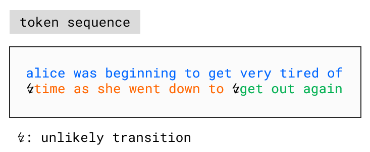
Few unlikely transitions can skew the average greatly.

A better approach could be to use the median, that is, the middle value of all sorted \(\phi_k\). Unlike the average, the median is resistant to skewing from a few highly unusual transitions. However, it can also be too inert: When the sequence consists of many short but mostly derivative blocks separated by unique transitions, the median would likely not reflect this at all, since it would remain dominated by the frequent common transitions within those blocks. A simple and practical solution to this is simply combining both, average \(\overline{\phi}_n\) and median \(\widetilde{\phi}_n\) as follows \[ \begin{align} \phi(s_0,\ldots,s_n)\, &:=\, (1 - \alpha)\, \overline{\phi}_n \,+\, \alpha\, \widetilde{\phi}_n \\[5px] &=\, \frac{1 - \alpha}{n} \sum_{k} \phi_k \,+\, \frac{\alpha}{2}\, \Big[\phi_{\big(\lfloor \frac{n+1}{2} \rfloor\big)} + \phi_{\big(\lceil \frac{n+1}{2} \rceil\big)}\Big] \end{align} \] where \(\alpha \in [0,1]\) and \(\phi_{(k)}\) is the \(k\)-th sorted value. I chose \(\alpha = 0.6\), giving the median a slightly stronger influence than the average. Implementing the final formula for \(\phi(s_0,\ldots,s_n)\) is straightforward and mainly involves computing each \(\phi_k\) i.e. the uniqueness of each transition \(s_{k-1} \to s_k\). To do this, first determine the specific weight of the edge connecting the vertex with ID1 to the vertex with ID2, then sum the weights of all outgoing edges from the vertex with ID1.

JS
                        const uniqueness = (ID1, ID2) => {
                            const edges = this.getEdges(ID1);

                            // corresponds to omega_(k-1)_k
                            const target = (edge) => edge.targetID.equals(ID2);
                            const choiceWeight = edges.find(target)?.weight || 0;

                            // corresponds to sum_j omega_(k-1)_j
                            const sumWeight = (sum, edge) => sum + edge.weight;
                            const totalWeight = edges.reduce(sumWeight, 0);

                            return 1 - choiceWeight / totalWeight;
                        };
                    
Calculating the uniqueness of a given transition.

Final Thoughts

Working on this project has been not only a lot of fun but also quite insightful. As promised in the beginning, we explored all the peripheral steps of systems like ChatGPT: From tokenization and handling large amounts of data to training and generation. I especially enjoyed implementing and applying Markov chains, as they, or stochastic processes in general, were among my favorite topics in university.

If this has sparked your curiosity and you'd like to learn more about the actual core of LLMs, that is neural networks, I encourage you to check out my other project on the classification of handwritten letters. If you have any questions or suggestions, feel free to contact me. Finally, thank you so much for reading all the way to the end!

philsfun.real@gmail.com plueschgiraffe